Many soil organic carbon (SOC) project developers see variance as a purely technical concern. In reality, variance is a key driver of uncertainty. Ignoring it can lead to undersampling, higher uncertainty deductions, and thus, reduced profitability.

At Seqana, we regularly encounter misconceptions about variance that can mislead even experienced project developers. In this post, we unpack the most common myths and offer practical guidance on how to understand and manage variance in your projects. 

What Is Variance and Why Does It Matter in SOC Projects?

Variance captures how much individual values deviate from their average. In SOC monitoring, it tells you how consistent or variable your carbon measurements are across space, over time, or between model predictions and ground truth.

The main ways variance shows up in carbon projects include:

• Spatial Variance of SOC Stock Snapshots: How much SOC levels vary between different locations at a single point in time. Relevant for independent (“unpaired") sampling.
  
  
• Variance of SOC Stock Change: How much the change in SOC stocks differs across locations between two time points. Relevant for paired sampling.
  
  
• Model Prediction Error Variance: How much predicted SOC stock or change values differ from field measurements across different locations.

Breaking variance down

Now let's build some intuition behind the numbers. Let’s say we’re measuring SOC in tons of carbon per hectare (tC/ha). The variance is in squared units (tC²/ha²), and it tells us how much measurements are spread out around the mean. 

‍

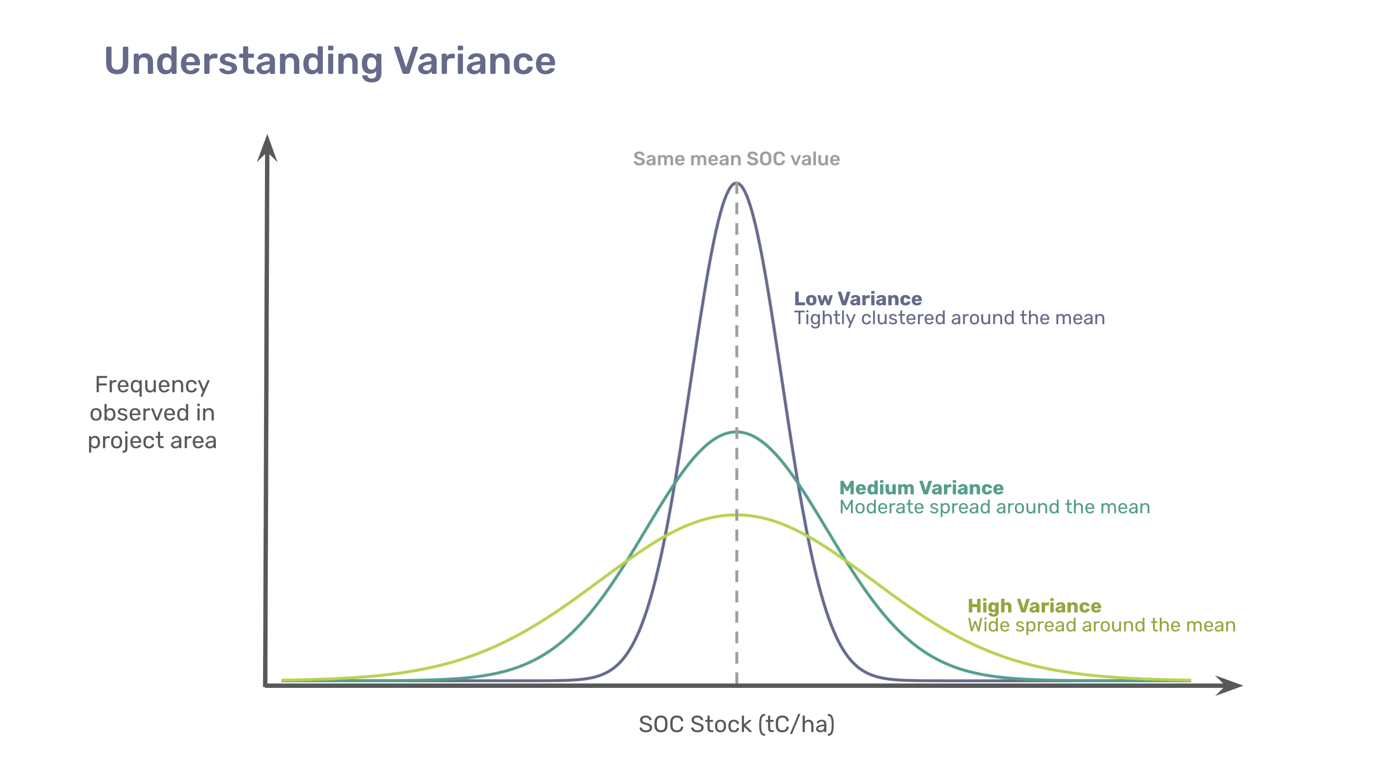
• Low Variance (e.g., below 150 tC²/ha² for spatial snapshot variance): Measurements are tightly clustered. If the average SOC stock is around 92 tC/ha, most values might fall between 85 and 100. It's worth noting that low variance does not mean low carbon stocks. It simply means that values are more consistent across the landscape.
  
  
• High Variance (e.g., 600 or more tC²/ha² for spatial snapshot variance): Measurements are more spread out. If the average SOC stock is still around 92 tC/ha, values might range more widely, for example from 50 to 135, showing a higher variance around the same mean.

The higher the variance, the more samples you need to detect meaningful differences in SOC stocks with confidence. Having a clear grasp of variance helps project developers make informed business-decisions around costs, project risks, and sampling designs.

Now that you have a foundational understanding of variance, let's dive into the most popular myths we've encountered in the market.

Myth 1: Variance depends on project size

It's tempting to assume that bigger projects must have a higher variance, but variance depends on heterogeneity of SOC stock, not the size of the project area.

‍

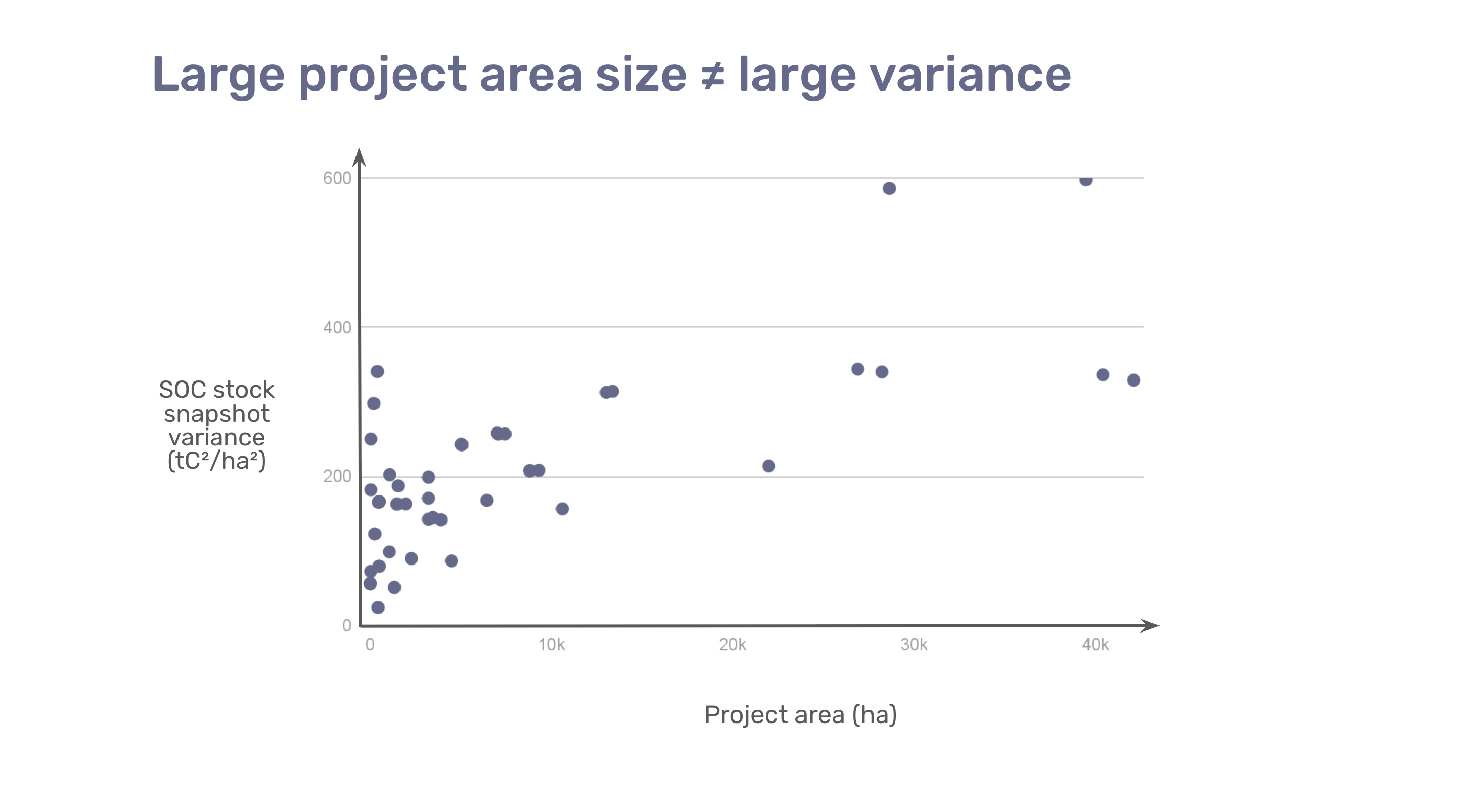
A small project with mixed land uses, multiple soil types, and diverse management histories can have higher variance than a large, uniform one. In fact, even smaller sections of a project often show higher variability than the overall project area. What matters most to the variance is the heterogeneity of the landscape and (historical) land use, not its size.

The range of SOC stock variance between projects can be substantial, and project size is not a reliable indicator. Despite this, some widely used frameworks, such as the FAO GSOC MRV protocol or the drafted EU Carbon Removal Certification Framework (CRCF), offer sample size guidelines based on project area, like “1 sample per 5 hectares.” While simple, this area-based approach misses the point: it’s not the size, but the variance that determines how many samples are needed. This makes it essential to estimate your project's variance directly. Otherwise, you risk under-sampling, which increases uncertainty deductions, or over-sampling, which unnecessarily increases sampling costs — both of which reduce your profits.

How Seqana estimates variance

At Seqana, we use a combination of data sources within machine learning models to accurately estimate variance:

• Proprietary soil sample database: Seqana maintains a growing internal database of over 1 million soil samples. These are used to train machine learning models that capture SOC stock variability across our clients project areas.
  
  
• Remote sensing and geospatial data: Satellite imagery, elevation models, and land cover information help identify patterns of variability in the landscape.
  
  
• Client-supplied preliminary data: When available, field samples from the project area can be used to validate and improve model performance.

Once variance is modeled, we use these insights to create a stratified sampling design, grouping project areas into relatively uniform zones to reduce within-stratum variance and improve sampling efficiency (see Seqana's approach to Sampling Design).

‍

Myth 2: There’s nothing I can do about variance

SOC stock variance, and the variance of SOC stock change, are both inherent features of the landscape, its climate, and management. While this variability can not be eliminated, what matters in the context of SOC projects is how much of the variance of SOC stock change can be explained through modeling.

The job of a model—whether process-based or statistical—is to explain as much of the landscape's variability as possible. Model performance is often summarized using a metric called R², or the coefficient of determination, where a value of 0 means the model explains none of the observed variation, and a value of 1 means it explains all of it. The more that a model captures real-world variation, the lower the uncertainty and associated uncertainty deductions will be.

In practice, no model is ever perfect. Even well-calibrated models typically explain only part of the total variation observed in SOC stock changes. This portion is known as the explained variance and reflects what the model is able to account for. The remaining portion is the unexplained variance (technically often referred to as “residual variance”), which represents the variation not captured by the model.

This distinction is critical for carbon accounting: only the unexplained variance contributes to uncertainty deductions. The better your model explains variance—through environmental covariates, historical data, or spatial structure—the less unexplained variance you must account for with conservative buffers or deductions. In other words, explaining variance is the key to reducing uncertainty.

Seqana’s approach is built around this principle. Our sampling design, and precision layers such as Digital Soil Maps (DSMs), all aim to explain as much variance as possible. By capturing the patterns that drive SOC variability—soil texture, topography, land use, etc.—we minimize the unexplained portion that would otherwise inflate uncertainty deductions. This directly translates into improved project economics through reduced uncertainty (deductions).

This process helps project developers build sampling strategies that reflect the true variance of the landscape rather than relying on assumptions based solely on area, which reduces sampling inefficiencies and strengthens alignment with project goals.

‍

Myth 3: “Close enough” is good enough

‍

‍

Paired sampling aims to measure SOC stock changes over time by revisiting the same sampling points. In this context, the relevant variance is that of the SOC stock change over time. However, practical constraints can turn what is assumed to be a variance of change into what is actually two spatial snapshots:

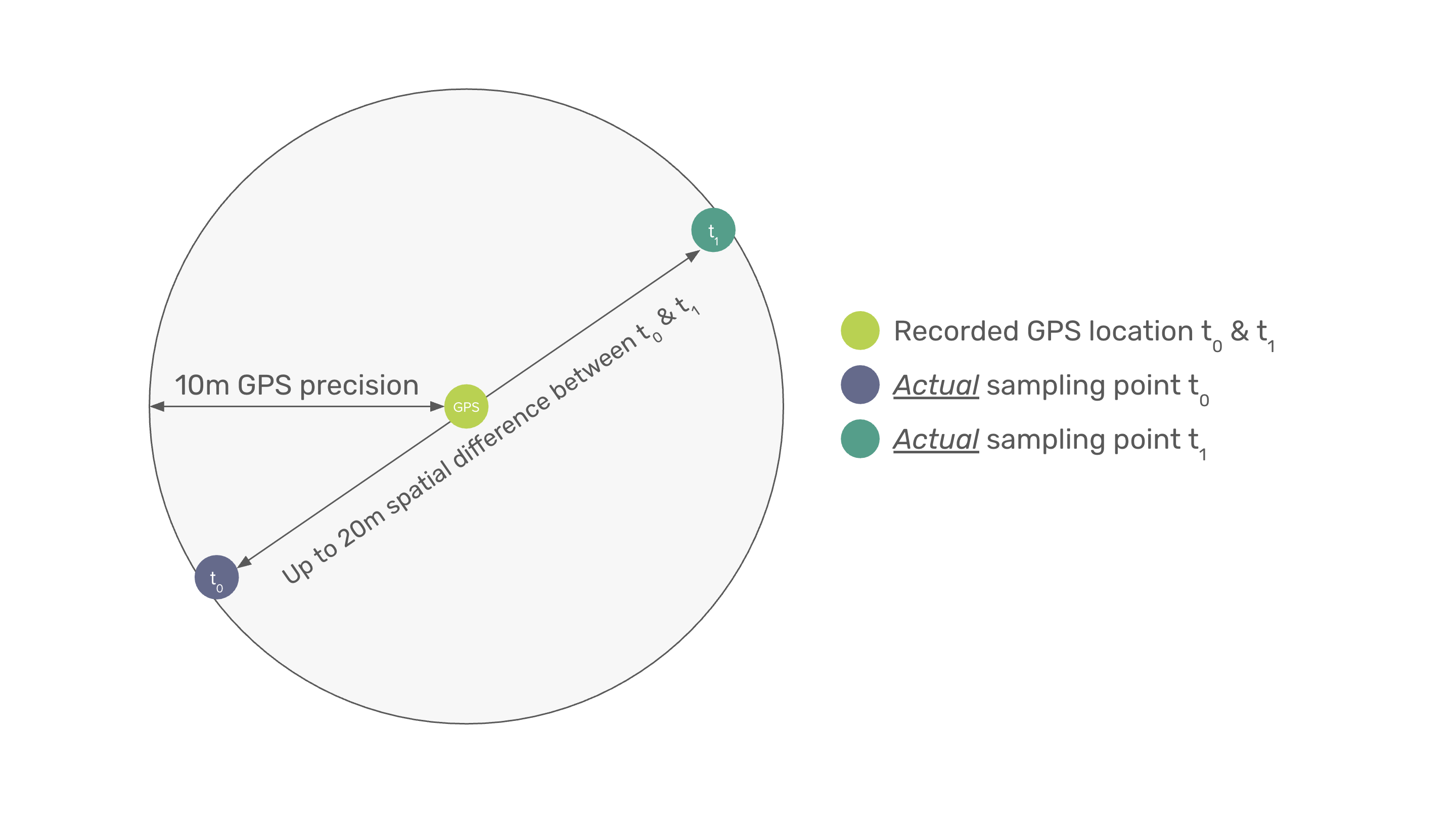
• Soil sampling is destructive, therefore, the original core cannot be resampled and analyzed in the future. In theory, true paired sampling requires the ability to sample the exact same core over time. In practice, resampling is conducted in close proximity to the original core (with the assumption that this serves as a valid proxy for the SOC stock and its change at the original location). However, this assumption can be problematic.
  
  
• GPS precision is typically limited to around 5–10 meters. This makes it difficult to resample the original sampling location.
  
  
• Even small distance shifts matter. Studies have shown that significant differences in SOC stocks (5-7 tC/ha) have been observed between samples just 40 cm apart—greater than typical multi-year SOC stock changes (Poeplau et al. 2022). 

These practical constraints mean that what is assumed to be a measure of variance of change may actually reflect spatial snapshot variance if the remeasurement is slightly off-location (and, strictly speaking, is not the same soil from the previous sampling). Misinterpreting this as a change in SOC over time can lead to false positives or false negatives.

The takeaway: Paired sampling can be a powerful tool, but it must be carefully designed and interpreted to distinguish actual changes from small-distance spatial variability. At Seqana, we help our clients address this variability and tailor their sampling strategy to the specific requirements of their project area. This includes guidance on whether to use individual cores or composite samples, as well as how many sub-samples to collect for composite sampling. To support these decisions, we conduct simulations to evaluate the trade-offs between uncertainty reduction and sampling costs—enabling us to deliver bespoke, data-driven recommendations for each sampling approach.

‍

The Reality: Variance shapes every stage of your project

Variance of SOC stock, SOC stock change, and of model errors influence every stage of a soil carbon project from budgeting to modeling and verification. Addressing variance early helps project developers reduce uncertainty, plan smarter, and maximize profits.

‍

Need help estimating or managing variance?

Seqana supports project developers in understanding and managing the variance of SOC stock and SOC stock change within their projects. We help quantify this variance through rigorous assessments and work to explain as much of it as possible using advanced modeling approaches, including Digital Soil Mapping (DSM) and Model-Assisted Estimation (MAE). By combining sound stratification and sampling design with strong predictive modeling, we help reduce uncertainty and the deductions that result from it. Whether you are designing a new project or preparing for verification, we are here to ensure you do so with confidence.

Contact us to talk through your variance strategy.

‍

References:

Poeplau, C., Prietz, R., & Don, A. (2022). Plot‑scale variability of organic carbon in temperate agricultural soils: Implications for soil monitoring. Journal of Plant Nutrition and Soil Science, 185(3), 403–416. https://doi.org/10.1002/jpln.202100393